Semantic Classification of Boundaries of an RGBD Image
Nishit Soni, Anoop M. Namboodiri, CV Jawahar and Srikumar Ramalingam. Semantic Classification of Boundaries of an RGBD Image. In Proceedings of the British Machine Vision Conference (BMVC 2015), pages 114.1-114.12. BMVA Press, September 2015. [paper] [abstract] [poster] [code] [bibtex]
Download the dataset from here.
Summary
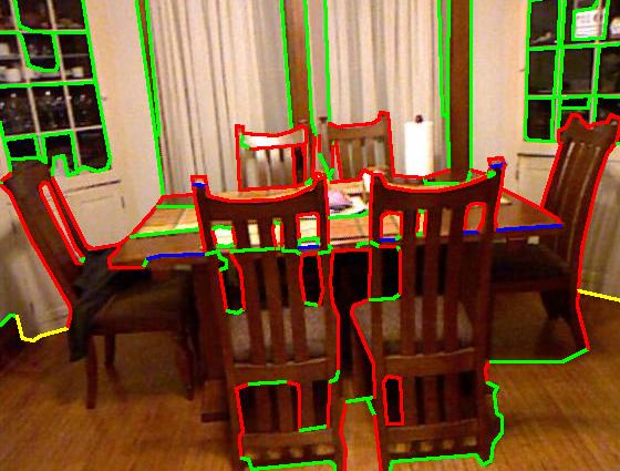
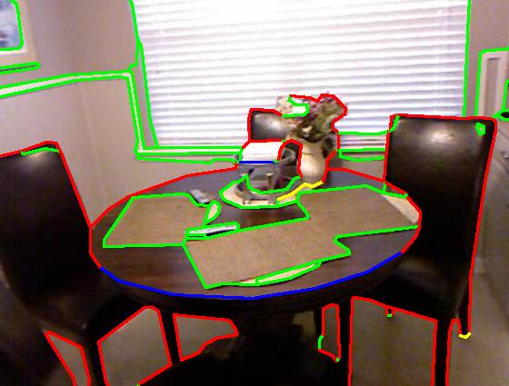
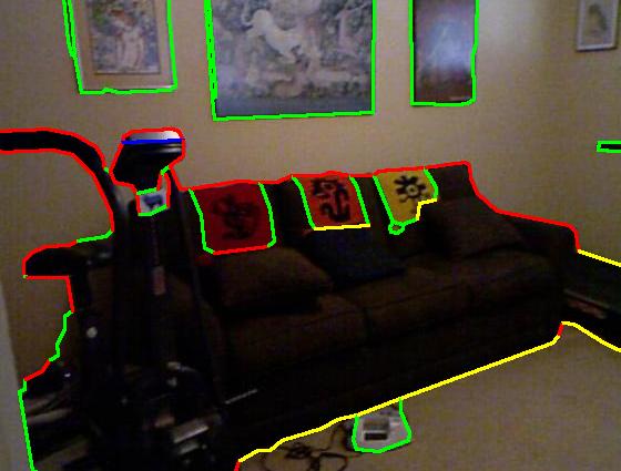
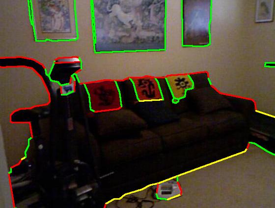
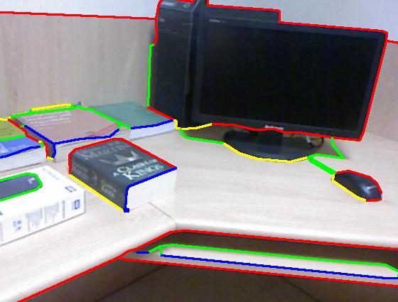
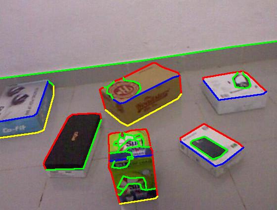
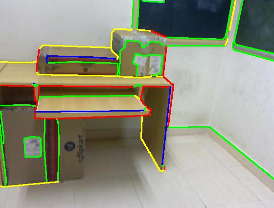
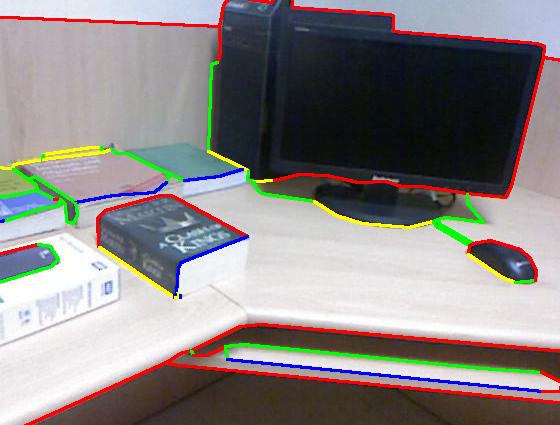
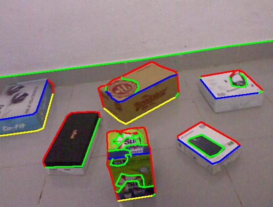
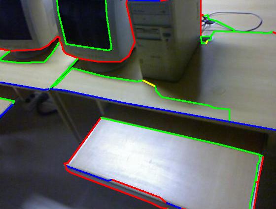
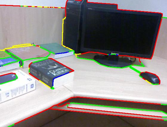
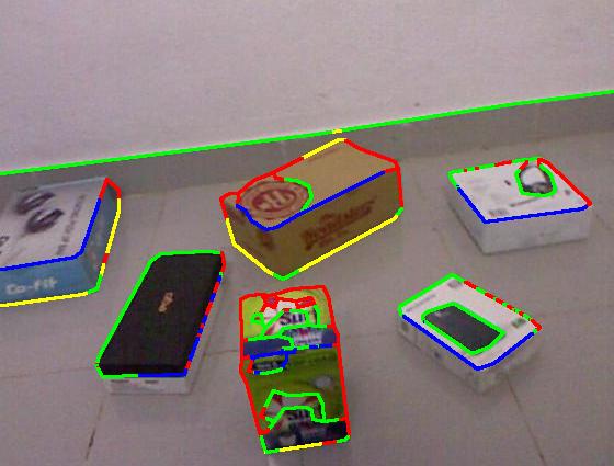
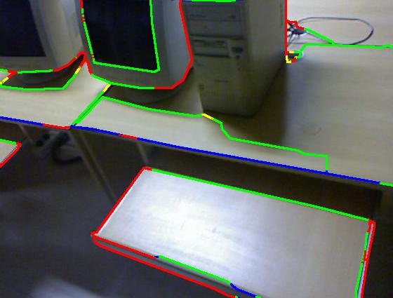
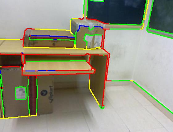
Edges in an image often correspond to depth discontinuities at object boundaries (occlusion edges) or normal discontinuities (convex or concave edges). In addition, there could be planar edges that are within planar regions. Planar edges may result from shadows, reflection, specularities and albedo variations. Figure 2 shows a sample image with edge labels. Figure 1 represents the kinect depth map of that image. This paper studies the problem of classifying boundaries from RGBD data. We propose a novel algorithm using random forest for classifying edges into convex, concave and occluding entities. We release a data set with more than 500 RGBD images with pixel-wise groundtruth labels. Our method produces promising results and achieves an F-score of 0.84.
We use both image and depth cues to infer the labels of edge pixels. We start with a set of edge pixels obtained from an edge detection algorithm and the goal is to assign one of the four labels to each of these edge pixels. Each edge pixel is uniquely mapped to one of the contour segments. Contour segments are sets of linked edge pixels. We formulate the problem as an optimization on a graph constructed using contour segments. We obtain unary features using pixel classifier based on Random forest. We design a feature vector with simple geometric depth comparison features. We use a simple Potts model for pairwise potentials. The individual steps in the algorithm is shown in figure 3.
Figure 3 : This figure summarizes the pipeline of our approach. It shows RGB and depth maps as input (1st image set), with Pb edge detection (2nd image). The classification and MRF outputs are shown in the last two images respectively. Color code: red (occluding), green (planar), blue (convex), yellow (concave).
Experiments and Results
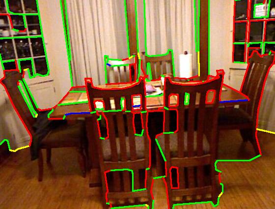
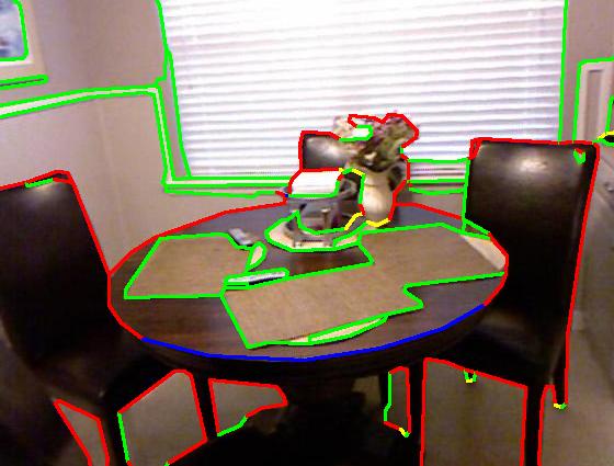
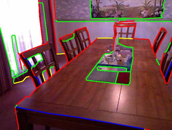
For quantitative evaluation of the method, we have created an annotated dataset of 500 RGBD images of varying complexity. Train to test ratio is 3:2. Our dataset consists of objects such as tables, chairs, cupboard shelves, boxes and household objects in addition to walls and floors. We also annotate 100 images from NYU dataset, which include varying scenes from bed-room, living-room, kitchen, bathroom and so on with different complexities.
We compare our approach with Gupta et al. [1] and show that our approach provides better results. The approach that we present here provides good labels for most pixels with high precision and the performance degrades when there is a significant loss in the depth data. We get an average F-score of 0.82 on the classification results for our data set. The use of smoothness constraints in the MRF achieves an F-score of 0.84. The NYU dataset contains complex scenes containing glass windows and table heads. We achieve an average F-score of 0.74 for the NYU dataset. Below is the quantitative evaluation of our approach along with the comparison with Gupta et al..
|
|
| Groundtruth | 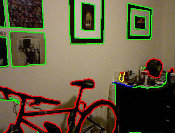 |
 |
 |
 |
 |
| Result | 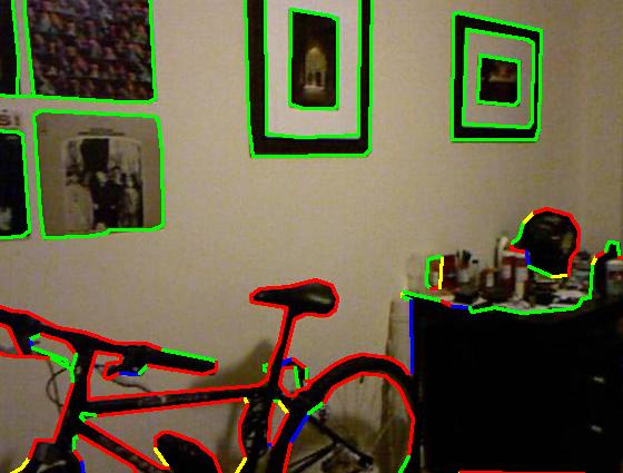 |
 |
 |
 |
 |
| Groundtruth | 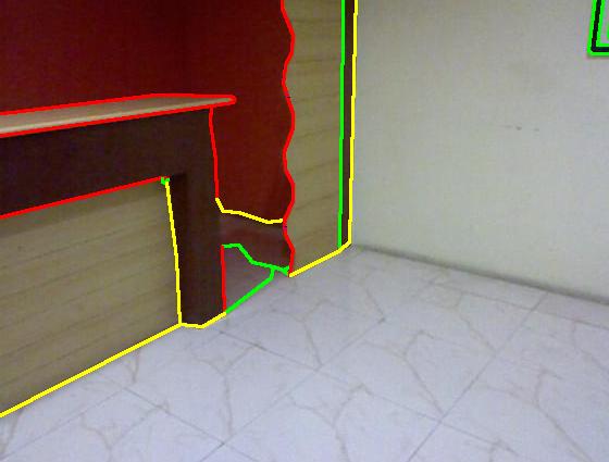 |
 |
 |
 |
 |
| Our result |  |
 |
 |
 |
 |
| Sgupta et al. [1] | 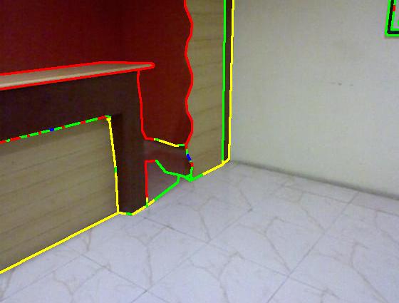 |
 |
 |
 |
 |
References
- S. Gupta, P. Arbelaez, and J. Malik. Perceptual organization and recognition of indoor scenes from rgb-d images. In CVPR, 2013.
Authors
Nishit Soni 1
Anoop M. Namboodiri 1
C. V. Jawahar 1
Srikumar Ramalingam 2
1 International Institute of Information Technology, Hyderabad.
2 Mitsubishi Electric Research Lab (MERL), Cambridge, USA.